
Chapter 3 : Classification
Notes
MNIST
- The MNIST dataset is a set of 70,000 small images of handwritten digits with labels
- This is probably the most used dataset for machine learning
from sklearn.datasets import fetch_openml
import numpy as np
# MNIST changed to https://www.openml.org/d/554
mnist = fetch_openml("mnist_784", version=1, as_frame=False)
# Do this to follow along with Geron
def sort_by_target(mnist):
    reorder_train = np.array(sorted([(target, i) for i, target in enumerate(mnist.target[:60000])]))[:, 1]
    reorder_test = np.array(sorted([(target, i) for i, target in enumerate(mnist.target[60000:])]))[:, 1]
    mnist.data[:60000] = mnist.data[reorder_train]
    mnist.target[:60000] = mnist.target[reorder_train]
    mnist.data[60000:] = mnist.data[reorder_test + 60000]
    mnist.target[60000:] = mnist.target[reorder_test + 60000]
mnist.target = mnist.target.astype(np.int8)
sort_by_target(mnist)
X, y = mnist["data"], mnist["target"]
print(X.shape, y.shape)
(70000, 784) (70000,)
%matplotlib inline
import matplotlib.pyplot as plt

dim = 28
some_num = 36_000
example = X[some_num]
plt.imshow(example.reshape((dim, dim)), cmap="binary")
plt.axis("off");
y[some_num]
5

Split into train / test!
X_train, y_train, X_test, y_test = X[:60000], y[:60000], X[60000:], y[60000:]
# Shuffling
shuf_order = np.random.permutation(len(y_train))
X_train, y_train = X_train[shuf_order, :], y_train[shuf_order]
Training a Binary Classifier
y_train_5 = (y_train == 5)
y_test_5 = (y_test == 5)
from sklearn.linear_model import SGDClassifier

sgd_clf = SGDClassifier()
sgd_clf.fit(X_train, y_train_5)
SGDClassifier()
sgd_clf.predict([example])
# This is sometimes False
array([ True])
Performance Measures
Measuring Accuracy Using Cross-Validation
from sklearn.model_selection import cross_val_score
cross_val_score(sgd_clf, X_train, y_train_5, cv=3, scoring="accuracy")
array([0.96835, 0.96025, 0.9659 ])
from sklearn.base import BaseEstimator

class Never5Classifier(BaseEstimator):
    def fit(self, X, y=None):
        return self
    def predict(self, X):
        return np.zeros((len(X), 1), dtype=bool)

n5c = Never5Classifier()
n5c.fit(X_train, y_train_5)
cross_val_score(n5c, X_train, y_train_5, cv=3, scoring="accuracy")
array([0.9102 , 0.9103 , 0.90845])
Misleading Performance Conclusions
- Results for our Stochastic Gradient Descent Classifier are ~95%!
- These results are ostensibly good, because only guessing False would be 90% accurate
- Thus, accuracy is not the preferred performance measure for classifiers, especially when data is skewed
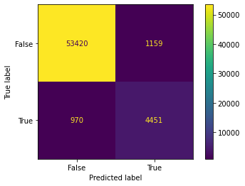
Confusion Matrix
- General idea is the count the number of times class A was classified as class B
from sklearn.model_selection import cross_val_predict

y_train_pred = cross_val_predict(sgd_clf, X_train, y_train_5, cv=3)
# This is a pretty useful function, what it does is
# Does the k-fold CV and notes the prediction in each fold (using the other
# as training data), then it stacks them all at the end
from sklearn.metrics import confusion_matrix, ConfusionMatrixDisplay
# Requires sklearn > 0.24
cmd = ConfusionMatrixDisplay.from_predictions(y_train_5, y_train_pred)
cm = cmd.confusion_matrix
This is a useful image for understanding this straight from Geron’s book:

Precision, Recall, and F1 Score
Precision
$ precision = \frac {TP}{TP + FP} $
When your classifier claims to predict a 5, it is correct precision % of the time.
Recall
$ recall = \frac {TP}{TP + FN} $
It only detects recall % of the 5’s.
$F_1$ Score
$ F_1 = \frac {2}{\frac{1}{precision} + \frac{1}{recall}} = \frac {TP}{TP + \frac{FN + TP}{2}} $
Harmonic mean of recall and precision. Both need to be high to get a high $F_1$ Score.
Precision/Recall Scenarios
- Scenario 1: Safe video classifier, if video is safe –> 1, else 0. We want high precision because we never want the model thinking that the video is safe, when in reality it is violent. And we don’t care if we block a decent amount of safe videos.
-
Scenario 2: Detect shoplifters on security footage, if shoplifting –> 1, else 0. We want high recall because we never want the model thinking that the person is not shoplifting, when in reality they are. And we don’t care if we occasionally accuse people of shoplifting that actually aren’t.
- Scenario 3: Taking a bet model, if you should bet –> 1, else 0. We want high precision because we never want to have the model predict a win, but the bet is actually a loss. Even at the price of missing out on a few good opportunities.
- Scenario 4: Will jumping off this structure kill me, if yes –> 1, else 0. We want high recall because we never want to predict that it won’t kill me, but in reality it would. Sorry for the grim example…
from sklearn.metrics import precision_score, recall_score, f1_score

print(precision_score(y_train_5, y_train_pred)) # 4766 / (4766 + 2121)
print(recall_score(y_train_5, y_train_pred))
print(f1_score(y_train_5, y_train_pred))
0.7934046345811052
0.8210662239439218
0.8069984588885868
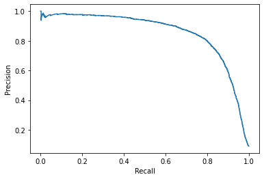
y_scores = cross_val_predict(sgd_clf, X_train, y_train_5, cv=3, method="decision_function")
from sklearn.metrics import precision_recall_curve

precisions, recalls, thresholds = precision_recall_curve(y_train_5, y_scores)
from sklearn.metrics import PrecisionRecallDisplay

# This is precision vs recall
disp = PrecisionRecallDisplay(precision=precisions, recall=recalls)
disp.plot()

# Geron's plot
def plot_precision_recall_vs_threshold(p, r, t):
    plt.plot(t, p[:-1], "b--", label="Precision")
    plt.plot(t, r[:-1], "g-", label="Recall")
    plt.xlabel("Threshold")
    plt.legend(loc="upper left")
    plt.ylim([0, 1])
plt.figure()
plot_precision_recall_vs_threshold(precisions, recalls, thresholds)
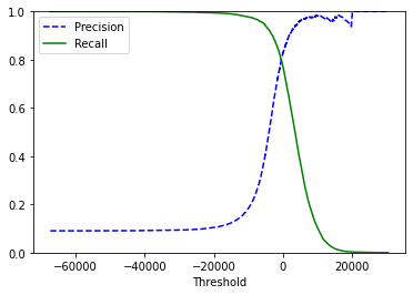
# My curve is much different...
thresh = min(thresholds[np.argwhere(precisions > 0.9)[:-1, 0]])
y_train_pred_90 = (y_scores > thresh)
print(precision_score(y_train_5, y_train_pred_90))
print(recall_score(y_train_5, y_train_pred_90))
0.9001540041067762
0.646928610957388
The ROC Curve
from sklearn.metrics import roc_curve

fpr, tpr, thresholds = roc_curve(y_train_5, y_scores)

def plot_roc_curve(fpr, tpr, label=None):
    plt.plot(fpr, tpr, lw=2, label=label)
    plt.plot([0, 1], [0, 1], "k--")
    plt.axis([0,1,0,1])
    plt.xlabel("False Positive Rate")
    plt.ylabel("True Positive Rate")

plot_roc_curve(fpr, tpr)
plt.show()
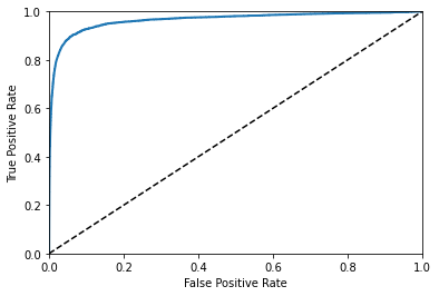
# ROC Area Under the Curve Score
from sklearn.metrics import roc_auc_score

roc_auc_score(y_train_5, y_scores)
0.9653886554659126
Rule of Thumb
Use PR Curve when positive class is rare and you care more about the false positives than the false negatives. Our classifier (which isn’t very good) looks good on the ROC curve, but that’s only because there’s only 10% 5s in the dataset (few positives).
from sklearn.ensemble import RandomForestClassifier

forest_clf = RandomForestClassifier()
y_probas_forest = cross_val_predict(forest_clf, X_train, y_train_5, cv=3, method="predict_proba")
y_scores_forest = y_probas_forest[:, 1]
fpr_forest, tpr_forest, thresholds_forest = roc_curve(y_train_5, y_scores_forest)
plt.plot(fpr, tpr, "b:", label="SGD")
plot_roc_curve(fpr_forest, tpr_forest, label="Random Forest")
plt.legend(loc="lower right")
<matplotlib.legend.Legend at 0x12ceeb6d0>
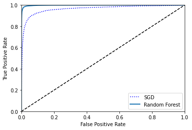
roc_auc_score(y_train_5, y_scores_forest) # Much better!!
0.9984537812756192
Multiclass Classification
- Some algorithms can handle multiple classes directly:
- Random Forest Classifiers
- Naive Bayes Classifiers
- Others are strictly binary classifiers
- Support Vector Machine Classifiers
- Linear Classifiers
- These can be converted to multiclassifers
- One-versus-all strategy (OvA)
- Create 10 binary classifiers and pick the one with the highest score
- One-versus-one strategy (OvO)
- Create classifiers to predict 0s vs 1s, 0s vs 2s, … 0s vs 9s, 1s vs 2s, 1s vs 3s, …
- Need N * (N - 1) / 2 classifiers
- Most of the time OvA is preferred
- Scikit-learn automatically runs OvA when you use a strictly binary classifier (except SVM where is uses OvO)
sgd_clf.fit(X_train, y_train)
sgd_clf.predict([example])
array([5], dtype=int8)
some_num_scores = sgd_clf.decision_function([example])
some_num_scores
array([[ -9769.65818671, -24825.69130821, -10776.58906031,
         -1405.53715487, -19212.67326423,   2556.83203592,
        -20584.60080404, -18743.62574742,  -8281.89554637,
        -12370.00869108]])
forest_clf.fit(X_train, y_train)
forest_clf.predict([example])
array([5], dtype=int8)
forest_clf.predict_proba([example])
array([[0.04, 0. , 0. , 0.05, 0. , 0.87, 0.03, 0. , 0. , 0.01]])
cross_val_score(sgd_clf, X_train, y_train, cv=3, scoring="accuracy")
array([0.88685, 0.89025, 0.8789 ])
from sklearn.preprocessing import StandardScaler
scaler = StandardScaler()
X_train_scaled = scaler.fit_transform(X_train)
cross_val_score(sgd_clf, X_train_scaled, y_train, cv=3, scoring="accuracy")
/Users/riley/PycharmProjects/ML/venv/lib/python3.8/site-packages/sklearn/linear_model/_stochastic_gradient.py:696: ConvergenceWarning: Maximum number of iteration reached before convergence. Consider increasing max_iter to improve the fit.
  warnings.warn(
/Users/riley/PycharmProjects/ML/venv/lib/python3.8/site-packages/sklearn/linear_model/_stochastic_gradient.py:696: ConvergenceWarning: Maximum number of iteration reached before convergence. Consider increasing max_iter to improve the fit.
  warnings.warn(
/Users/riley/PycharmProjects/ML/venv/lib/python3.8/site-packages/sklearn/linear_model/_stochastic_gradient.py:696: ConvergenceWarning: Maximum number of iteration reached before convergence. Consider increasing max_iter to improve the fit.
  warnings.warn(


array([0.9016 , 0.90595, 0.90815])
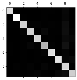
Error Analysis
# Look at the confusion matrix
y_train_pred = cross_val_predict(sgd_clf, X_train_scaled, y_train, cv=3)
conf_mx = confusion_matrix(y_train, y_train_pred)
conf_mx
/Users/riley/PycharmProjects/ML/venv/lib/python3.8/site-packages/sklearn/linear_model/_stochastic_gradient.py:696: ConvergenceWarning: Maximum number of iteration reached before convergence. Consider increasing max_iter to improve the fit.
  warnings.warn(
/Users/riley/PycharmProjects/ML/venv/lib/python3.8/site-packages/sklearn/linear_model/_stochastic_gradient.py:696: ConvergenceWarning: Maximum number of iteration reached before convergence. Consider increasing max_iter to improve the fit.
  warnings.warn(


array([[5606,    0,   14,    7,    9,   48,   36,    5,  197,    1],
       [   0, 6434,   43,   20,    3,   45,    4,   10,  173,   10],
       [  30,   27, 5250,   87,   80,   29,   71,   41,  335,    8],
       [  24,   22,  110, 5260,    1,  213,   30,   44,  359,   68],
       [  10,   17,   40,    8, 5265,   11,   34,   22,  272,  163],
       [  27,   17,   30,  159,   53, 4520,   78,   19,  456,   62],
       [  30,   18,   49,    1,   36,  102, 5557,    9,  116,    0],
       [  20,   14,   50,   22,   47,   13,    6, 5725,  145,  223],
       [  19,   65,   46,   97,    3,  132,   28,    8, 5399,   54],
       [  23,   19,   30,   58,  123,   37,    1,  167,  296, 5195]])
plt.matshow(conf_mx, cmap="gray")
<matplotlib.image.AxesImage at 0x12d08fb20>
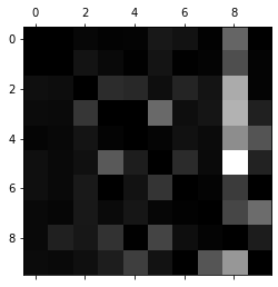
row_sums = conf_mx.sum(axis=1, keepdims=True)
norm_conf_mx = conf_mx / row_sums
np.fill_diagonal(norm_conf_mx, 0)
plt.matshow(norm_conf_mx, cmap="gray")
<matplotlib.image.AxesImage at 0x12d1a9a90>
Multilabel Classification
- A classification system that outputs multiple binary labels is a multilabel classification system
- Picture with Alice and Charlie should output
[1, 0, 1]
from sklearn.neighbors import KNeighborsClassifier

y_train_large = (y_train >= 7)
y_train_odd = (y_train % 2 == 1)
y_multilabel = np.c_[y_train_large, y_train_odd]

knn_clf = KNeighborsClassifier()
knn_clf.fit(X_train, y_multilabel)
KNeighborsClassifier()
knn_clf.predict([example])
array([[False, True]])
# Typo in book here y_train --> y_multilabel
# Takes a long time
# y_train_knn_pred = cross_val_predict(knn_clf, X_train, y_multilabel, cv=3, n_jobs=-1)
# f1_score(y_multilabel, y_train_knn_pred, average="macro")
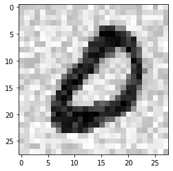
Multioutput Classification
- Generalization of the multilabel classification where each classification can be multiple labels and each label can have multiple classifications/outputs
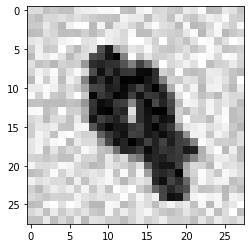
# Noise removal classifier
import numpy.random as rnd
train_noise = rnd.randint(0, 100, (len(X_train), 784))
test_noise = rnd.randint(0, 100, (len(X_test), 784))
X_train_mod = X_train + train_noise
X_test_mod = X_test + test_noise
y_train_mod = X_train
y_test_mod = X_test
plt.imshow(X_train_mod[some_num].reshape((28, 28)), cmap="binary")
plt.show()
plt.imshow(y_train_mod[some_num].reshape((28, 28)), cmap="binary")
<matplotlib.image.AxesImage at 0x12c401e50>
knn_clf.fit(X_train_mod, y_train_mod)
clean_digit = knn_clf.predict([X_test_mod[5000]])
plt.imshow(X_test_mod[5000].reshape((28, 28)), cmap="binary")
plt.show()
plt.imshow(clean_digit.reshape((28, 28)), cmap="binary")
<matplotlib.image.AxesImage at 0x12d771b50>
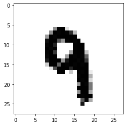
That turned out pretty nice. Let’s go a step further and use this as input to model
new_in = []
for i in range(0, len(X_train_mod), 1000):
    print(i)
    new_in.append(knn_clf.predict(X_train_mod[i:i+1000, :]))
0
1000
2000
3000
4000
5000
6000
7000
8000
9000
10000
11000
12000
13000
14000
15000
16000
17000
18000
19000
20000
21000
22000
23000
24000
25000
26000
27000
28000
29000
30000
31000
32000
33000
34000
35000
36000
37000
38000
39000
40000
41000
42000
43000
44000
45000
46000
47000
48000
49000
50000
51000
52000
53000
54000
55000
56000
57000
58000
59000
new_inn = np.vstack(new_in)
new_inn.shape
(60000, 784)
cross_val_score(sgd_clf, new_inn, y_train, cv=3, scoring="accuracy", verbose=4, n_jobs=4)
[Parallel(n_jobs=4)]: Using backend LokyBackend with 4 concurrent workers.
[Parallel(n_jobs=4)]: Done   3 out of   3 | elapsed:  1.4min remaining:    0.0s
[Parallel(n_jobs=4)]: Done   3 out of   3 | elapsed:  1.4min finished


array([0.9067 , 0.9008 , 0.90305])
# Eh, ok, so it was about the same