Chapter 5 : Support Vector Machines

Linear SVM Classification

• This chapter is about Support Vector Machines which are capable of performing linear or nonlinear classification, regression, and even outlier detection
• They are well suited for classification of complex but small- or medium-sized datasets

The following image represents an SVM (on the right) vs. linear classifiers (left) on the Iris dataset:

You can think of an SVM classifier as fitting the widest possible street between the classes. This is called large margin classification. Adding more training instances will not affect the decision boundary at all. The dashed lines in the right plot are the support vectors which form the edge of the street. SVMs are very sensitive to feature scales.

Soft Margin Classification

• Hard margin classification is when we impose the condition that all classifications are separated by a single line
  • This isn’t possible if the data is not linearly separable
  • It’s very sensitive to outliers
• To avoid these pitfalls soft margin classification is used
• The goals of soft margin classification are:
  • Make the street as wide as possible
  • Limit the number of margin violations
• The balance of these goals is controlled by the C hyperparameter. Smaller C values lead to a wider street, but more margin violations.
• If your SVM model is overfitting you can try reducing C to have it generalize better

Nonlinear SVM Classification

• Not all datasets are linearly separable
• You can sometimes add features (the example Geron uses is squaring a variable x where abs(x) < 2 is positive, else negative classification)

Polynomial Kernel

• Adding low order polynomial features like won’t work with very complex datasets
• And if high order polynomial features are added then the model becomes too slow

The Kernel Trick

Geron didn’t really explain this all that much. But, here is a really good explanation of the kernel trick. Basically, instead of squaring, cubing, etc. each feature and concatenating them as a new feature, using a kernel allows you to compute the square, cube, etc. of each feature from just the original features. Thus, it saves computational time.

import matplotlib.pyplot as plt
import numpy as np
from sklearn.svm import SVC
from sklearn.pipeline import Pipeline
from sklearn.preprocessing import StandardScaler
from sklearn.datasets import make_moons

X, y = make_moons(n_samples=100, noise=0.15, random_state=42)


def plot_dataset(X, y, axes):
    plt.plot(X[:, 0][y == 0], X[:, 1][y == 0], "bs")
    plt.plot(X[:, 0][y == 1], X[:, 1][y == 1], "g^")
    plt.axis(axes)
    plt.grid(True, which="both")
    plt.xlabel(r"$x_1$", fontsize=20)
    plt.ylabel(r"$x_2$", fontsize=20, rotation=0)


poly_kernel_svm_clf = Pipeline(
    [
        ("scaler", StandardScaler()),
        ("svm_clf", SVC(kernel="poly", degree=3, coef0=1, C=5)),
    ]
)
poly_kernel_svm_clf.fit(X, y)

poly_kernel_svm_clf10 = Pipeline(
    [
        ("scaler", StandardScaler()),
        ("svm_clf", SVC(kernel="poly", degree=10, coef0=5, C=5)),
    ]
)
poly_kernel_svm_clf10.fit(X, y)


def plot_predictions(clf, axes):
    x0s = np.linspace(axes[0], axes[1], 100)
    x1s = np.linspace(axes[2], axes[3], 100)
    x0, x1 = np.meshgrid(x0s, x1s)
    X = np.c_[x0.ravel(), x1.ravel()]
    y_pred = clf.predict(X).reshape(x0.shape)
    y_decision = clf.decision_function(X).reshape(x0.shape)
    plt.contourf(x0, x1, y_pred, cmap=plt.cm.brg, alpha=0.2)
    plt.contourf(x0, x1, y_decision, cmap=plt.cm.brg, alpha=0.1)


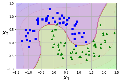
plot_predictions(poly_kernel_svm_clf, [-1.5, 2.5, -1, 1.5])
plot_dataset(X, y, [-1.5, 2.5, -1, 1.5])
plt.figure()
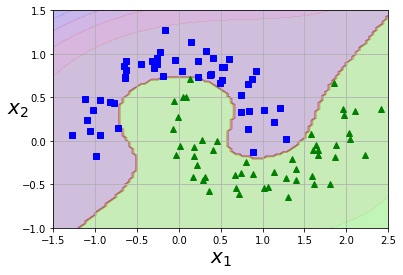
plot_predictions(poly_kernel_svm_clf10, [-1.5, 2.5, -1, 1.5])
plot_dataset(X, y, [-1.5, 2.5, -1, 1.5])

Adding Similarity Features

A similarity function such as the Gaussian Radial Basis Function (RBF) can be used to add features which help increase dimensionality. This transform a one dimension feature into two dimensions by comparing the distance to landmarks within the dataset. How to select landmark? In an ideal world you’d try all possible landmarks, but that would increase the feature matrix to m x m.

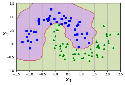
Gaussian RBF Kernel

You can once again use the kernel trick with the RBF.

rbf_kernel_svm_clf = Pipeline(
    [("scaler", StandardScaler()), ("svm_clf", SVC(kernel="rbf", gamma=10, C=100))]
)
rbf_kernel_svm_clf.fit(X, y)
plot_predictions(rbf_kernel_svm_clf, [-1.5, 2.5, -1, 1.5])
plot_dataset(X, y, [-1.5, 2.5, -1, 1.5])

Rules of thumb when picking kernels

• Grid search is your friend
• Try linear kernel first
• If the training set is not too large, try Gaussian RBF kernel
• Then try others if you have more time

Computational Complexity

• LinearSVC does not support the kernel trick, but scales linearly with the number of samples and features
• SVC supports the kernel trick, but becomes slow (O(m^3 x n)) with a large number of samples

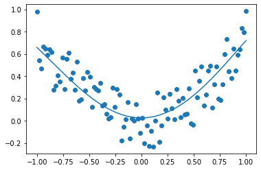
SVM Regression

• Instead of trying to fit the largest possibile street between two classes while limiting margin violations, SVM Regression tries to fit as many instances as possible on the street while limiting margins violations (ones off the street)
• You can use LinearSVR to perform linear SVM regression

from sklearn.svm import LinearSVR

X = np.linspace(-1, 1, 100).reshape((-1, 1))
X = np.hstack((X, X**2))
y = 0.75 * X[:, 0] ** 2 + 0.5 * (np.random.random(X.shape[0]) - 0.5)
svm_reg = LinearSVR(epsilon=0.01, fit_intercept=True, verbose=True, max_iter=10000)
svm_reg.fit(X, y)
print(svm_reg.__dict__)
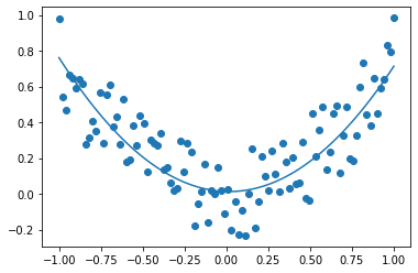
plt.scatter(X[:, 0], y)
plt.plot(X[:, 0], svm_reg.predict(X))

[LibLinear]{'tol': 0.0001, 'C': 1.0, 'epsilon': 0.01, 'fit_intercept': True, 'intercept_scaling': 1.0, 'verbose': True, 'random_state': None, 'max_iter': 10000, 'dual': True, 'loss': 'epsilon_insensitive', 'n_features_in_': 2, 'coef_': array([-0.02389477,  0.72415554]), 'intercept_': array([0.01291348]), 'n_iter_': 484}





[<matplotlib.lines.Line2D at 0x125a30a30>]

from sklearn.svm import SVR

svm_poly_reg = SVR(kernel="poly", degree=2, C=100, epsilon=0.1)
svm_poly_reg.fit(X, y)
plt.scatter(X[:, 0], y)
plt.plot(X[:, 0], svm_poly_reg.predict(X))

[<matplotlib.lines.Line2D at 0x125a80dc0>]

Note

• SVMs can also be used for outlier detection

Under the Hood

• Decision function for the SVM classifier is 0 when the weights * input_data + bias is less than 0 and 1 otherwise
• So the decision line is where weights * input_data + bias = 0
• There’s a slack term added to the soft margin linear SVM classifier objective

Quadratic Programming

• https://web.stanford.edu/~boyd/cvxbook/bv_cvxbook.pdf

The Dual Problem

• Primal problem - a constrained optimization problem
• Dual problem - a problem related to the primal problem whose solution typically gives a lower bound to the primal problem solution (sometimes can have the same solution)
• In the SVM case the solutions to the primal problem and dual problem are equivalent
• The dual problem is faster to solve than the primal when the number of training instances is smaller than the number of features (rare)
• The dual problem makes the kernel trick possible

Kernelized SVM

• See explanation of the kernel trick above, basically allows you get the benefit of transforming and creating new features without having to do so explicitly
• Kernel - is a function capable of computing the dot product of $\phi(\textbf{a})^T \cdot \phi(\textbf{b})$ based only on the original vector $\textbf{a}$ and $\textbf{b}$, without any dependence on the transformation $\phi$.

Online SVMs

• It’s possible to use Gradient Descent to minimize the cost function in Equation 5-13, but it converges much more slowly than the methods based on QP

• Felt like this was an important image in understand why we minimize norm(w), because the lower the slope of the decision plane, the greater the margin will be dividing the data classes

Hinge Loss

\(max(0, 1 - t)\)