Chapter 7 : Ensemble Learning and Random Forests

• A group of predictors is called an ensemble
• An ensemble of decision trees is known as a Random Forest
• This so called wisdom of the crowd approach of combining multiple models into an ensemble (or even multi ensembles of models) account for some of the best solutions in Machine Learning
• Popular ensemble methods include bagging, boosting, stacking, and more

Voting Classifiers

• A voting classifier uses the predictions of multiple diverse predictors (models) and has each one vote and then picks the majority vote
• This is called a hard voting classifier
• You can achieve high accuracy from a bunch of weak learners
• “Suppose you build an ensemble containing 1,000 classifiers that are individually correct only 51% o the time (barely better than random guessing). If you predict the majority voted class, you can hope for up to 75% accuracy!”
• However in practice this is only true if the classifiers are all independent of one another, which isn’t the case since they were all trained on the same data
• Ensemble methods work best when the predictors are as independent from one another as possible (e.g. use different training algorithms). This will allow them to make different types of errors, increasing the models accuracy.
• Soft voting is when you use predictors which have the predict_proba method (i.e. they predict probabilities). You pick the class with the highest class probability, averaged over all the individual classifiers. This is often more effective because it gives higher weight to higher confidence votes, whereas in hard voting they are all equally weighted (even though some individual models may be unconfident in the result).

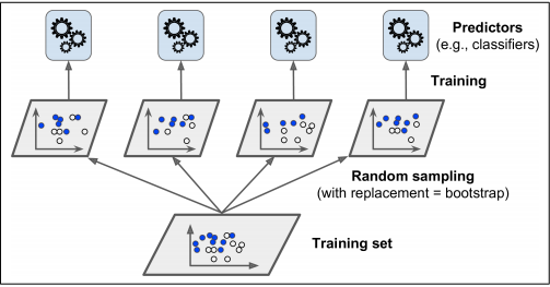
Bagging and Pasting

• Instead of using completely different algorithms to produce an ensemble model, another way to do so is to train the same algorithm on different random subsets of the training set
• This technique is known as bagging and pasting
• Bagging (short for bootstrap aggregating) is when you sample randomly from the training set with replacement
• Pasting is when you sample randomly from the training set without replacement

• The statistical mode is used for aggregating votes
• This aggregation reduces both bias and variance
• Generally the ensemble has a similar bias, but a lower variance than a single predictor trained on the original training set
• These methods scale very well

Bagging and Pasting in Scikit-Learn

%%script echo skipping
# What this looks like:
from sklearn.ensemble import BaggingClassifier
from sklearn.tree import DecisionTreeClassifier

bag_clf = BaggingClassifier(DecisionTreeClassifier(), n_estimators=500, max_samples=100, 
                            bootstrap=True, # False would be w/o replacement
                           n_jobs=4)
bag_clf.fit(X_train, y_train)
y_pred = bag_clf.predict(X_test)

skipping

• Bootstrapping introduces a bit more diversity in the subsets that each predictor is trained on
  • Bagging ends up with a slightly higher bias than pasting, but thisalso means that predictors end up being less correlated so the ensemble’s variance is reduced
• Overall, bagging often results in better models, which explains why it is generally preferred
• You can evalute both bagging and pasting if you have time

Out-of-Bag Evaluation

• https://stats.stackexchange.com/questions/88980/why-on-average-does-each-bootstrap-sample-contain-roughly-two-thirds-of-observat
• https://stats.stackexchange.com/questions/173520/random-forests-out-of-bag-sample-size
• If you sample randomly with replacement it turns out that for each predictors about 37% of the samples will not be selected (for large enough number of samples m)
• These unsampled samples are known as out-of-bag instances
• Thus by performing validation on the oob instances and averaging across predictors we can get an estimate of the accuracy on the test set
• So it serves as like a free validation set oob_score=True

Random Patches and Random Subspaces

• Random Patches - Sampling both training instances and features
• Random Subspaces - Keeping all training instances, but sampling features

Random Forests

• Generally trained via bagging, typically with max_samples set to the size of the training set
  • This means if your training set has M samples. Pick a random number between 1 and M. Select that sample. Pick another random sample in this way. Do that M times. As explained above, roughly 37% of the samples will not be selected.
• You can wrap DecisionTreeClassifier in a BaggingClassifier or just use RandomForestClassifier, the hyperparameters are roughly the same

Extra Trees

• When growing a random forest at each node only a subset of features is considered for splitting
• Extremely Randomized Tree ensemble (AKA Extra Trees) - when instead of using the “best” (purest) threshold for each node, a tree building algorithm uses random thresholds for each feature
• Extra Trees are much less costly to generate because it doesn’t need to spend time calculating the loss of all the features at each node.
• It’s difficult to tell which will do better (RandomForestClassifer or ExtraTreesClassifier) a priori

Feature Importance

• In a single Decision Tree important features are likely to appear near the root of the tree
  • Recall that if at each node all features are analyzed to see which will be split the data, therefore if one feature will split the data better we should expect it to appear near the root
• Scikit-learn keeps track of this in the feature_importances_ variable
• This is a huge bonus!

from sklearn.datasets import load_iris
from sklearn.ensemble import RandomForestClassifier
iris = load_iris()
rnd_clf = RandomForestClassifier(n_estimators=500, n_jobs=4)
rnd_clf.fit(iris["data"], iris["target"])
for name, score in zip(iris["feature_names"], rnd_clf.feature_importances_):
    print(name, score)

sepal length (cm) 0.10260569493424748
sepal width (cm) 0.025482769522540718
petal length (cm) 0.4238524136066159
petal width (cm) 0.44805912193659586

Boosting

• Boosting or Hypothesis Boosting refers to any Ensemble method that can combine several weak learners into a strong learner
• The general idea of most boosting methods is to train predictors sequentially, each trying to correct its predecessor
• XGBoost or AdaBoost
• The general idea of AdaBoost is to refit the training instances which were underfit by the predecessor
• New predictions focus more and more on hard cases
• Here’s an example where the weights of missed classification instances are increased by each successive model:
• The traditional base estimator for Adaboost is a stump, which is a decision tree with just one node and two leaves
• If AdaBoost is overfitting the training set, try reducing the number of estimators or more strongly regularizing the base estimator

Gradient Boosting

• The difference between Adaboost and Gradient Boosting is that instead of increasing the weights of missed prediction in the predecessor estimator, gradient boosting tries to fit the residual errors of the predecessor
• The code for gradient boosting is as follows

%%script echo skipping
from sklearn.tree import DecisionTreeRegressor

tree_reg1 = DecisionTreeRegressor(max_depth=2)
tree_reg1.fit(X, y)
y2 = y - tree_reg1.predict(X)
tree_reg2 = DecisionTreeRegressor(max_depth=2)
tree_reg2.fit(X, y2)
y3 = y2 - tree_reg2.predict(X)
tree_reg3 = DecisionTreeRegressor(max_depth=2)
tree_reg3.fit(X, y3)
# ...
y_pred = sum(tree.predict(X_new) for tree in (tree_reg1, tree_reg2, tree_reg3))

skipping

• A simpler way to train GBRT ensembles is to use GradientBoostingRegressor

%%script echo skipping
# Equivalent to above example
from sklearn.ensemble import GradientBoostingRegressor

gbrt = GradientBoostingRegressor(max_depth=2, n_estimators=3, learning_rate=1.0)
gbrt.fit(X, y)

skipping

• How many tree should you have and what should be the learning rate?
  • You can use early stopping to determine the hyper parameters which produce the best results on the validation set

%%script echo skipping
import numpy as np
from sklearn.model_selection import train_test_split
from sklearn.metrics import mean_squared_error

X_train, X_val, y_train, y_val = train_test_split(X, y, random_state=49)

gbrt = GradientBoostingRegressor(max_depth=2, n_estimators=120, random_state=42)
gbrt.fit(X_train, y_train)

errors = [mean_squared_error(y_val, y_pred)
          for y_pred in gbrt.staged_predict(X_val)]
bst_n_estimators = np.argmin(errors) + 1

gbrt_best = GradientBoostingRegressor(max_depth=2, n_estimators=bst_n_estimators, random_state=42)
gbrt_best.fit(X_train, y_train)

# Or

gbrt = GradientBoostingRegressor(max_depth=2, warm_start=True, random_state=42)

min_val_error = float("inf")
error_going_up = 0
for n_estimators in range(1, 120):
    gbrt.n_estimators = n_estimators
    gbrt.fit(X_train, y_train)
    y_pred = gbrt.predict(X_val)
    val_error = mean_squared_error(y_val, y_pred)
    if val_error < min_val_error:
        min_val_error = val_error
        error_going_up = 0
    else:
        error_going_up += 1
        if error_going_up == 5:
            break  # early stopping

skipping

Stacking

• Stacking - short for stacked generalization uses a model to make the final prediction instead of just taking the majority vote from a bunch of weak learners
• The final predictor is called a blender or meta learner
• First divide the training set into two subsets (1 and 2)
  • The first subset is used to train the individual predictors (weak learners)
  • Once that’s done they make predictions on the second subset to produce a clean dataset of predicted values
  • Those predicted values are used as inputs into the blender with the same targets
• You can do this several times over and form several layers
• Scikit-learn doesn’t have an implementation of this, but see DESlib