NFL Matchup Modeling

November 2020

Introduction - Disclaimer
Methodology
- Points Prediction: Convolved PDFs
Shortcomings

Introduction

Disclaimer

This isn’t intended to be a rigorous or valid analysis I was just playing around.

The NFL consists of 16 regular season games. Each week teams battle it out on the field while oddsmakers in Vegas are determined to set lines that will be bet equally on both sides. Traditionally, the three most common betting lines are:

Moneyline - The team that will win the game.
Spread - The differential between the favored team’s score and the underdog.
Over/Under - The total number of points in the game.

As an example, here are the current lines for an upcoming game this weekend (Week 10):

Example Game Lines

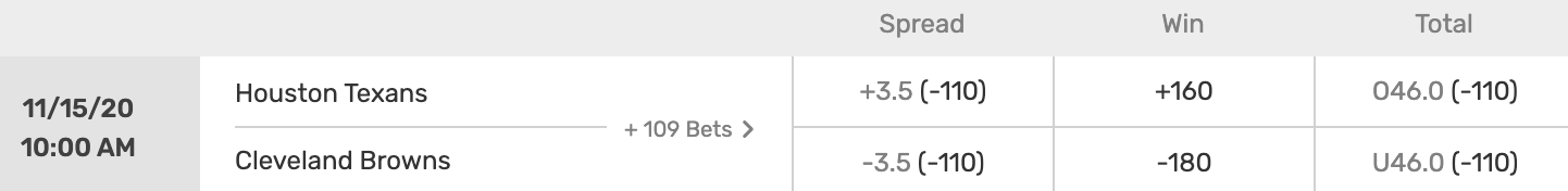
The goal of this project is to use mathematical methods and analysis to correctly predict the winning side, the spread, and total points.

Methodology

Points Prediction: Convolved PDFs

The idea behind this approach is simple (dumb). Let’s say we would like to know the number of points team 1 will score against team 2. Consider the distribution of points scored by the team 1 offense in preceding weeks. Consider the distribution of points surrendered by the team 2 defense in preceding weeks. Sticking with the matchup above:

Week	1	2	3	4	5	6	7	8	9
Houston Texans’s Points Scored	20	16	21	23	30	36	20	BYE	27
Houston Texans’s Points Surrended	34	33	28	31	14	42	35	BYE	25

>>> 
Score Scraper
 
        
        
            Code

import requests
from bs4 import BeautifulSoup as bs
import pandas as pd

team = "Houston Texans"
base_url = "https://www.pro-football-reference.com/years/2020/week_{}.htm"
max_week = 9

offensive_scores = []
defensive_scores = []
for week in range(1, max_week + 1):
    url = base_url.format(week)
    r = requests.get(url)
    soup = bs(r.text, "html.parser")
    games = soup.find_all(attrs={"class": "teams"})
    offensive_score = defensive_score = "BYE"
    for game in games:
        table_rows = game.find_all("td")
        for i, tr in enumerate(table_rows):
            if tr.string in [team]:
                offensive_team = tr.string
                offensive_score = int(table_rows[i + 1].string)
                try:
                    # Hacky
                    defensive_team = table_rows[i + 3].string
                    defensive_score = int(table_rows[i + 4].string)
                except IndexError:
                    defensive_team = table_rows[i - 3].string
                    defensive_score = int(table_rows[i - 2].string)
                offensive_scores.append(offensive_score)
                defensive_scores.append(defensive_score)
    if offensive_score == "BYE":
        offensive_scores.append(offensive_score)
        defensive_scores.append(defensive_score)

indexes = [f"{team}'s Points Scored", f"{team}'s Points Surrended"]
# columns = list(map(lambda x: f"Week {x}", range(1, max_week + 1)))
columns = list(range(1, max_week + 1))
values = [offensive_scores, defensive_scores]
df = pd.DataFrame(index=indexes, columns=columns, data=values)
print(df.to_markdown(tablefmt="github"))
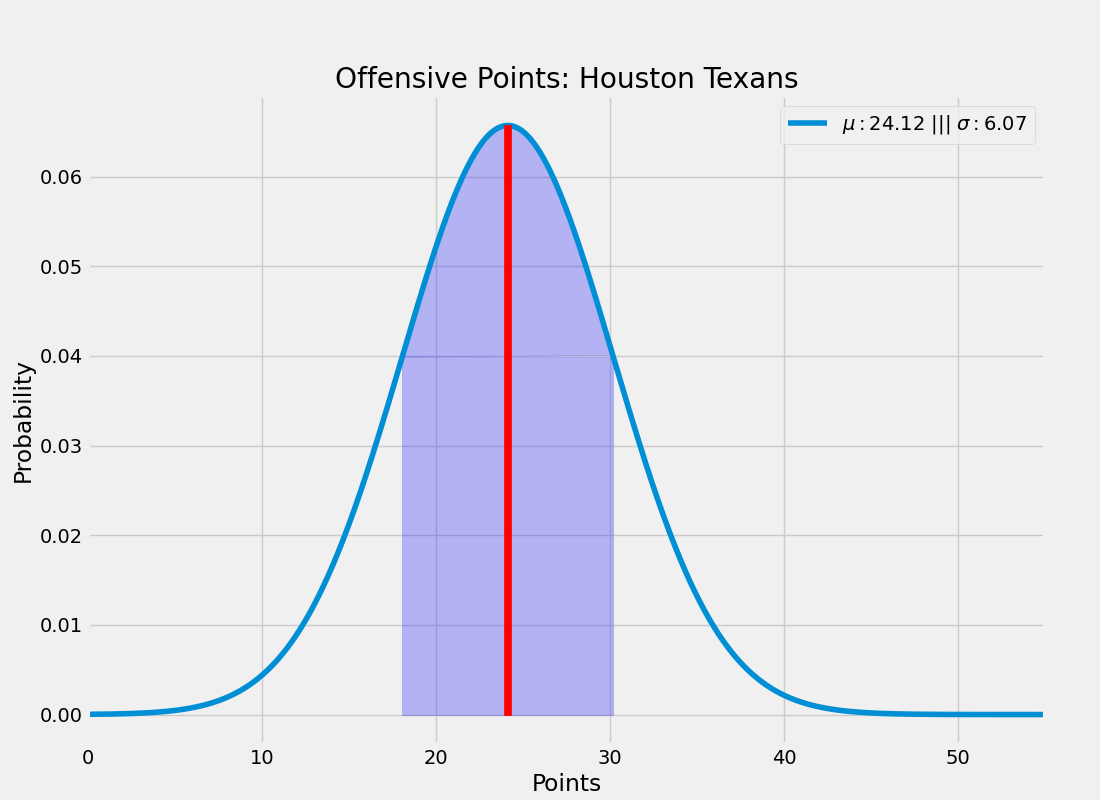
print(offensive_scores)

This is just a distribution of numbers so from its mean and standard deviation we can form a Gaussian:

Example Gaussian

>>> 
Offensive Points Gaussian PDF
 
        
        
            Code

import os
from scipy.stats import norm
from scipy.interpolate import interp1d
from scipy.integrate import quad
import numpy as np
import matplotlib
import matplotlib.pyplot as plt
matplotlib.rcParams["figure.figsize"] = (11, 8)
plt.style.use('fivethirtyeight')

scores = [20, 16, 21, 23, 30, 36, 20, 'BYE', 27]
scores = [i for i in scores if isinstance(i, int)]

team = "Houston Texans"
xmin = 0
xmax = 55



def make_pdf(x, y):
    # This sucks, but this is the only way I can think to do this...
    f = interp1d(x, y, kind="cubic")
    tot = quad(f, xmin, xmax)
    mu = quad(lambda x1: x1 * f(x1), xmin, xmax)[0]
    std = np.sqrt(quad(lambda x1: (x1 - mu) ** 2 * f(x1), xmin, xmax))[0]
    return y / tot[0], mu, std



def plot_offensive_points(scores):
    mean = np.mean(scores)
    std = np.std(scores)
    x = np.linspace(xmin, xmax, 1000)
    y = norm.pdf(x, mean, std)
    y, _, _ = make_pdf(x, y)
    plt.plot(x, y, label=f"$\mu: {mean : .2f}$ ||| $\sigma : {std : .2f}$")
    w = 0.2
    mask = (mean - std < x) & (mean + std > x)

    plt.fill(x[mask], y[mask], alpha=0.25, color="blue")
    plt.fill_between([mean - std, mean + std], min(y[mask]), color="blue", alpha=0.25)
    plt.fill_between([mean - w, mean + w], max(y[mask]), color="red", zorder=100)
    plt.legend()
    plt.xlim(left=0, right=55)
    plt.xlabel("Points")
    plt.ylabel("Probability")
    plt.title(f"Offensive Points: {team}")
    rel_path = "assets/images/nfl-matchup-modeling/gaussian1.png"
    p = os.path.abspath(os.getcwd())
    for i in range(3):
        p = os.path.dirname(p)
    plt.savefig(os.path.relpath(os.path.join(p, rel_path)))


plot_offensive_points(scores)

Now consider the distribution of points surrendered by the Cleveland Browns defense:

Week	1	2	3	4	5	6	7	8	9
Cleveland Browns’s Points Scored	38	30	20	38	23	38	34	16	BYE

>>> 
Score Scraper (Browns Defense)
 
        
        
            Code

import requests
from bs4 import BeautifulSoup as bs
import pandas as pd

team = "Cleveland Browns"
base_url = "https://www.pro-football-reference.com/years/2020/week_{}.htm"
max_week = 9

offensive_scores = []
defensive_scores = []
for week in range(1, max_week + 1):
    url = base_url.format(week)
    r = requests.get(url)
    soup = bs(r.text, "html.parser")
    games = soup.find_all(attrs={"class": "teams"})
    offensive_score = defensive_score = "BYE"
    for game in games:
        table_rows = game.find_all("td")
        for i, tr in enumerate(table_rows):
            if tr.string in [team]:
                offensive_team = tr.string
                offensive_score = int(table_rows[i + 1].string)
                try:
                    # Hacky
                    defensive_team = table_rows[i + 3].string
                    defensive_score = int(table_rows[i + 4].string)
                except IndexError:
                    defensive_team = table_rows[i - 3].string
                    defensive_score = int(table_rows[i - 2].string)
                offensive_scores.append(offensive_score)
                defensive_scores.append(defensive_score)
    if offensive_score == "BYE":
        offensive_scores.append(offensive_score)
        defensive_scores.append(defensive_score)

indexes = [f"{team}'s Points Scored"]
# columns = list(map(lambda x: f"Week {x}", range(1, max_week + 1)))
columns = list(range(1, max_week + 1))
values = [defensive_scores]
df = pd.DataFrame(index=indexes, columns=columns, data=values)
print(df.to_markdown(tablefmt="github"))
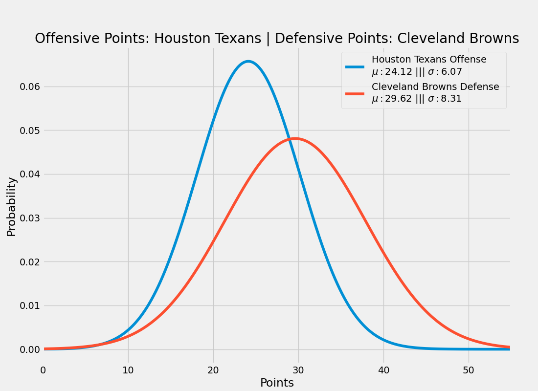
print(defensive_scores)

Combining these together we get the following Gaussian distributions:

Matchup Distribution

>>> 
Matchup Distribution
 
        
        
            Code

import os
from scipy.stats import norm
from scipy.interpolate import interp1d
from scipy.integrate import quad
import numpy as np
import matplotlib
import matplotlib.pyplot as plt
matplotlib.rcParams["figure.figsize"] = (11, 8)
plt.style.use('fivethirtyeight')

offensive_scores = [20, 16, 21, 23, 30, 36, 20, 'BYE', 27]
offensive_scores = [i for i in offensive_scores if isinstance(i, int)]
defensive_scores = [38, 30, 20, 38, 23, 38, 34, 16, 'BYE']
defensive_scores = [i for i in defensive_scores if isinstance(i, int)]


team1 = "Houston Texans"
team2 = "Cleveland Browns"
xmin = 0
xmax = 55

def save_path():
    fname = os.path.abspath(__file__)
    fname = os.path.split(fname)[-1].replace(".py", ".png")
    rel_path = f"assets/images/nfl-matchup-modeling/{fname}"
    p = os.path.abspath(os.getcwd())
    for i in range(3):
        p = os.path.dirname(p)
    return os.path.relpath(os.path.join(p, rel_path))

def make_pdf(x, y):
    # This sucks, but this is the only way I can think to do this...
    f = interp1d(x, y, kind="cubic")
    tot = quad(f, xmin, xmax)
    mu = quad(lambda x1: x1 * f(x1), xmin, xmax)[0]
    std = np.sqrt(quad(lambda x1: (x1 - mu) ** 2 * f(x1), xmin, xmax))[0]
    return y / tot[0], mu, std

def return_pdf_params(scores):
    mean = np.mean(scores)
    std = np.std(scores)
    x = np.linspace(xmin, xmax, 1000)
    y = norm.pdf(x, mean, std)
    y, _, _ = make_pdf(x, y)
    return x, y, mean, std

def plot_individual(x, y, mean, std):
    plt.plot(x, y, label=f"$\mu: {mean : .2f}$ ||| $\sigma : {std : .2f}$")



def plot_matchup_distributions():
    x1, y1, mean1, std1 = return_pdf_params(offensive_scores)
    x2, y2, mean2, std2 = return_pdf_params(defensive_scores)
    plt.plot(x1, y1, label=f"{team1} Offense \n$\mu: {mean1 : .2f}$ ||| $\sigma : {std1 : .2f}$")
    plt.plot(x2, y2, label=f"{team2} Defense \n$\mu: {mean2 : .2f}$ ||| $\sigma : {std2 : .2f}$")

    plt.legend()
    plt.xlim(left=0, right=55)
    plt.xlabel("Points")
    plt.ylabel("Probability")
    plt.title(f"Offensive Points: {team1} | Defensive Points: {team2}")
    plt.savefig(save_path())


plot_matchup_distributions()

For those who are not familiar with convolutions, it essentially will morph two waveforms together. This means that should a dominant offense (30 points per game (ppg)) play a weak defense (surrenders 40 ppg), the resulting waveform will predict the offense scoring more than usual (~35 points). However, if they play a strong defense (surrenders 20 ppg), then the expected offensive score will be lower (somewhere between ~25 points). If they play a defense which typically surrenders 30 ppg, then the convolution will support this expectation.

Convolution

>>> 
Convolution
 
        
        
            Code

import os
from scipy.stats import norm
from scipy.interpolate import interp1d
from scipy.signal import convolve
from scipy.integrate import quad
import numpy as np
import matplotlib
import matplotlib.pyplot as plt
matplotlib.rcParams["figure.figsize"] = (11, 8)
plt.style.use('fivethirtyeight')

offensive_scores = [20, 16, 21, 23, 30, 36, 20, 'BYE', 27]
offensive_scores = [i for i in offensive_scores if isinstance(i, int)]
defensive_scores = [38, 30, 20, 38, 23, 38, 34, 16, 'BYE']
defensive_scores = [i for i in defensive_scores if isinstance(i, int)]


team1 = "Houston Texans"
team2 = "Cleveland Browns"
xmin = 0
xmax = 55

def save_path():
    fname = os.path.abspath(__file__)
    fname = os.path.split(fname)[-1].replace(".py", ".png")
    rel_path = f"assets/images/nfl-matchup-modeling/{fname}"
    p = os.path.abspath(os.getcwd())
    for i in range(3):
        p = os.path.dirname(p)
    return os.path.relpath(os.path.join(p, rel_path))

def make_pdf(x, y):
    # This sucks, but this is the only way I can think to do this...
    f = interp1d(x, y, kind="cubic")
    tot = quad(f, xmin, xmax)
    mu = quad(lambda x1: x1 * f(x1), xmin, xmax)[0]
    std = np.sqrt(quad(lambda x1: (x1 - mu) ** 2 * f(x1), xmin, xmax))[0]
    return y / tot[0], mu, std

def return_pdf_params(scores):
    mean = np.mean(scores)
    std = np.std(scores)
    x = np.linspace(xmin, xmax, 1000)
    y = norm.pdf(x, mean, std)
    y, _, _ = make_pdf(x, y)
    return x, y, mean, std




def plot_matchup_distributions():
    x1, y1, mean1, std1 = return_pdf_params(offensive_scores)
    x2, y2, mean2, std2 = return_pdf_params(defensive_scores)
    plt.plot(x1, y1, label=f"{team1} Offense \n$\mu: {mean1 : .2f}$ ||| $\sigma : {std1 : .2f}$")
    plt.plot(x2, y2, label=f"{team2} Defense \n$\mu: {mean2 : .2f}$ ||| $\sigma : {std2 : .2f}$")

    values = convolve(y1, y2)
    x = np.linspace(xmin, xmax, len(values))
    values, mu, std = make_pdf(x, values)
    values, mu, std = make_pdf(x, values)
    plt.plot(x, values, label=f"Convolution: \n$\mu: {mu : .2f}$ ||| $\sigma : {std : .2f}$")

    plt.legend()
    plt.xlim(left=0, right=55)
    plt.xlabel("Points")
    plt.ylabel("Probability")
    plt.title(f"Offensive Points: {team1} | Defensive Points: {team2}")
    plt.savefig(save_path())


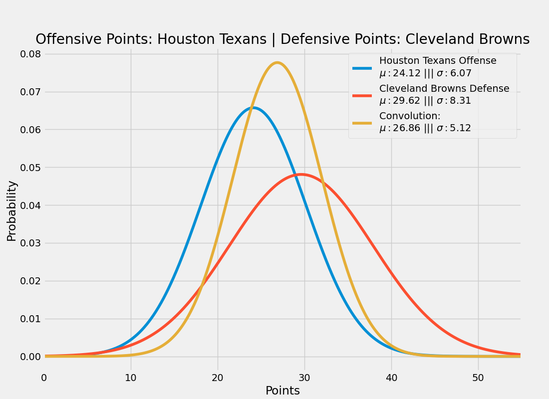
plot_matchup_distributions()

So this expects the Houston Texans to score 27 +/- 5 points against the Cleveland Browns this weekend.

Shortcomings

If you know anything about the upcoming matchup I’ve been running with you would think that’s crazy. Here are some reasons why:

First and foremost:

The Weather Channel is calling for an 80 percent chance of rain in Cleveland on Sunday, with 25-35 mph winds and occasional gusts over 50 mph.

Clearly this model does not account for inclement weather.
Large standard deviations. If the distribution of points is “too wide”, then it has trouble predicting a blowout more one sided result.
No recency bias. The Colts have come a long way since their week 1 woes. What you showed me last week matters much more than week one.
Personnel considerations. The Cowboys lost Dak and Dalton over the past few weeks. Jerry is picking guys off the street to fill their QB spot. Big Ben might be out with COVID.
It doesn’t account for the strength of the defenses you played. The way to the think about this is imagine a t1 which has only played lousy defenses. This t1 puts up 40 points a game. Their offense isn’t that good, they’ve just been playing high school defenses. Then they go to Pittsburgh and play the hard nosed Steelers, even if the model is saying they will put up less points than usual, they will probably put up much less because they haven’t played a real defense. I think this is the most accessible aspect to address, just takes some careful thought.
Doesn’t work for no prior data. Guess I’m sticking to my gut for week 1 picks next year. 😩
There’s no evidence this is how reality actually is. See Disclaimer.

Last time it was windy in Cleveland 😂

WINDY

Home

About

Projects

Posts